Create a Status Report with Green Checks and Red Flags in Excel

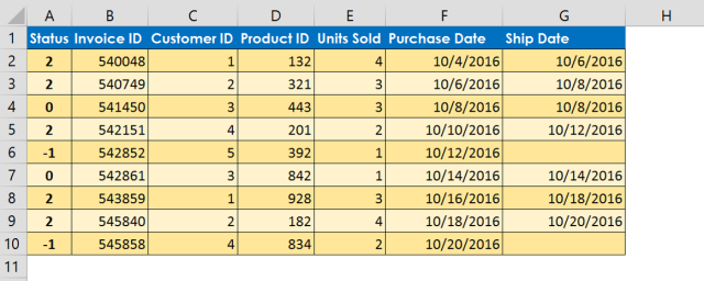
Let’s say that we have a spreadsheet that records a purchase date for when a customer places an order and a ship date for when the product ships out. We would like to have a red flag in column A for orders that currently have not been shipped. And if the product has shipped we would like a green check mark. See the below the example and then keep reading and I’ll show you how to create this spreadsheet using either Excel 2007, 2010, 2013 or 2016. Note that row 6 and row 10 displays a red flag because those orders have not been shipped.

Step 1: Click in cell A2 and write a formula =IF(G2=””,-1,G2-F2). This IF function checks if the Ship Date is blank. Excel an verify if there is a blank cell by using the formula =”” so if G2=”” is true then make the value equal to -1. Otherwise, if the ship date is not blank, then use the formula to equal ship date minus purchase date [G2-F2]. The answer will be zero if the order has the same ship date as the purchase date. Note that on row 4 and row 7 that the formula equals zero because the ship date is equal to the purchase date which results in 0.

Step 2: Copy the formula down using the auto fill handle.

Step 3: With the status cells selected in column A, choose the Conditional Formatting command from the Home tab. Select the icon sets menu and then click the 3 symbols (Uncircled).

Step 4: Click Conditional Formatting –> manage rules –> Edit formatting rule.

Step 5: Click show icon only (Screen shot below is from Excel 2013. Will look a little different in Excel 2007)

Step 6: Green check mark icon when value is >=0 Number. (Replace percent with number from the type drown down). Type a zero in the value area.

Step 7: Click no cell icon for when < 0 and >=0 Number. ( the middle range yellow exclamation mark will be replaced with no cell icon.

Step 8: Change the red X with a red flag for when <0 and click OK.

Click here to download this practice file.

Download my Excel Keyboard Shortcuts here.

 

 

 

 

 

Building PivotTable Reports Using Excel’s Data Model in Power Pivot with DAX formulas

Data Modeling Steps in Excel Power Pivot

1.Import data into Power Pivot Data Model

2.Create relationships between the Dimension Tables and Fact Tables

3.Create DAX formulas (Data Analysis Expressions)

• DAX Measures are used in the Values area of a PivotTable
• Calculated Columns are used in the criteria for Rows, Columns, and Slicers

4.Hide Tables and Fields not to be used in the PivotTables reports

5.Create PivotTables & PivotCharts

6.Refresh when source data changes

7.Update the Data Model if necessary

 

 

 

 

 

How to Use the IF Function and the VLOOKUP Function Together In Excel

The Vlookup function is an awesome function. It looks up information in a table where you have defined the lookup value in the left-most column of the table. In this video I share how to use it with an IF function after determining whether an individual has made their sales goal to determine their commission check.

Practice with my training file here. Also you might be interested in using the Match and Index functions as an alternative to the Vlookup if you have a large list of table columns.

Download my Excel Keyboard Shortcuts guide here.

How to Use the People Graph in Excel

The People Graph is an Excel 2013/2016 Add-In which makes graphic style charts. Find this command in the Add-Ins group of the Insert tab. Below is a video demonstration.

 

Automatically Update the Date and Time Stamp for Access Modified Records

Link an Excel Chart to a PowerPoint Presentation

In this post I will share with you how to link an Excel chart to a PowerPoint presentation. This is helpful when you expect changes to be made to the Excel chart and you want to have your audience view those changes from in one of your PowerPoint slides.

1. Right click the edge of the Excel chart and select copy.

2. Navigate to PowerPoint slide and select the Paste Special menu from the clipboard group.

 

3. Select Paste Link as Microsoft Excel Chart Object

4. Click File >Info and then click “Edit Links to Files” which is in the bottom right corner of PowerPoint 2010, 2013, and 2016 versions. Check box for “Automatic Update” in the Links box.

Note: It is important that the Excel file is saved to a location in which the PowerPoint can read the link otherwise the update cannot work. Typically you would save the Excel file with the chart to a network drive that is accessible to the file from which the PowerPoint is saved.

 

Click here to download my PowerPoint shortcuts.

 

Understanding Visio’s Glue to Shape vs Glue to Connection Point

In this post, I am going to explain how to connect Visio shapes. You can connect to the shape or to its connection point.

 

Format Red Cells if the Date is Older than One Year in Excel [Video]

In this video, I will demo how to format rows with red formatting if the date has been more than a year old. I will use the DATEDIF function to work within the conditional formatting rules.

 

 

 

Create a PivotTable in Excel [Video]

In this video, I will demo how to create an Excel PivotTable. This PivotTable will have Slicers and Timeline filters as well as a PivotTable chart.

 

A Special Trick to Select All Cells within the Find Box [Video]

This video will share with you how to search for cells within Excel’s find command and then select all the contents simultaneously.

In the video, I show you how to delete all rows that contain the same value. I use Excel’s find (control + F), type what I want to select. Then I click “find all”). The secret is to do control + A to select all.